ct3d — 3-D sparse-view parallel-beam CT

At a glance
Problem	3-D sparse-view parallel-beam CT of every axial slice (rotation about z)
Unknown	attenuation μ(x, y, z) ∈ [0, 1] (bounded head), 64 × 64 × 32
Physics	slice-stacked differentiable Radon transform: all slices × views in one grid_sample, exact autograd adjoint
Measurement	sinogram stack (views × detectors × slices), 30 views over 180° + 1 % noise; data on a 2× grid with 4 sub-rays per bin, float64
Difficulty classes	ellipsoids, blobs, piecewise
Baselines	fbp3d, grid (+ TV), deep_decoder
Metrics	PSNR · slice SSIM · MSE · IoU
Run	nefi run ct3d --smoke · full: nefi run configs/ct3d_full.yaml --device cuda

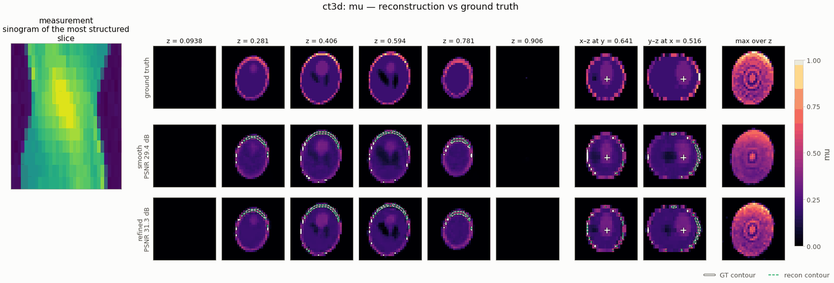
Gallery run (32 × 32 × 16, 12 views; 800 steps, 7.3 s on a CPU): PSNR 29.4 dB; edge refinement accepted, IoU 0.75 → 0.80. Rotate it in the 3-D showcase.

Recover a volumetric attenuation map μ(x, y, z) ∈ [0, 1] from n_views noisy parallel-beam projections of every axial slice: the source–detector pair rotates about the z axis, so the measurement is a stack of sinograms (n_views, n_det, n_z). With a few tens of views (a fraction of the ≈ π/2 · n an unregularized reconstruction needs) filtered back-projection streaks, and with a limited angular range (angle_range < 180°, the "missing wedge") it smears — the regime where the neural-field prior plus TV pays off.

CT3DScenes (ellipsoids | blobs | piecewise) ─► Radon3D on a 2× grid (4 sub-rays / bin, float64) ─► sinograms (V, n_det, n_z) + 1 % noise
coords ─► annealed Fourier PE (3-D) ─► MLP ─► Bounded(0, 1) ─► μ ─► Radon3D (all slices × views, one grid_sample)
       ─► MSE + λ·TV₃D(μ) ─► two-stage multiscale (½ res → native) ─► PSNR / slice-SSIM / MSE / feature IoU

from nefi.instances.ct3d import CT3D

inst = CT3D(preset="smoke")                 # 32×32×16, 12 views, 150 + 250 steps (≈ 6 s, one core)
out = inst.run(seed=0, device="cpu")
print(out.metrics)                          # psnr, ssim, mse, iou
fbp = inst.fbp(out.measurement)             # slice-wise FBP of the same sinogram stack

CLI: nefi run ct3d --smoke, nefi run configs/ct3d_full.yaml --device cuda, nefi bench ct3d --smoke --methods neural,fbp3d,grid. Example: python examples/ct3d.py [--set scene=piecewise --set angle_range=120] writes ct3d.png (z-slices and an x-z cut of GT / NF / FBP3D / |error|), sinogram.png, metrics.json, result.pt under runs/ct3d_smoke/.

Forward model (nefi.instances.ct3d.radon3d)

Radon3DOperator(domain, n_views, field="mu", angles=None, angle_range=π, det_per_pixel=1, samples_per_pixel=1, view_batch=None, max_samples=2**24) applies the 2-D rotation-based Radon transform of sparse_view_ct (same conventions, physical line integrals Δt Σ μ) to every slice — in one F.grid_sample call: the slices are the channels of a single (n_z, n, n) image and the rotated (n_t, n_det) sampling lattices of all views are stacked along the output height. There is no Python loop over slices or views; view_batch (automatic under max_samples gathered samples) chunks the views to bound memory at paper scale. Linear (homogeneity = 1), batchable, exact autograd adjoint (op.adjoint(y)), at_resolution keeps det_per_pixel so n_det scales with the lateral grid while the slices follow n_z: coarse curriculum data are area averages over detector bins and slices, which is exact for line integrals, so no custom downsampling is needed.

• fbp3d(sinogram, angles, filter="ramp", n=None, width=1, circle=False) / op.fbp(...) — slice-wise filtered back-projection (Kak & Slaney ramp, optional apodization), batched like the forward (all rows filtered at once, one grid_sample for the smearing);
• backproject3d(...) / op.backproject(y) — pixel-driven back-projector (independent discretization of Rᵀ).

Scenes and data

CT3DScenes (normalized coordinates, inside the scanner cylinder, cell-averaged with render_factor sub-samples per voxel and axis so the native ground truth is the exact area average of the 2× data-generation volume):

• ellipsoids — 3-D Shepp–Logan-like head: the 10-ellipsoid table of Kak & Slaney's 3-D phantom with the Toft contrasts (SHEPP_LOGAN_3D, ZXZ Euler angles), random global scale / rotation about z / shift and per-ellipsoid axes, centers, angles, intensities (the skull shell shares one perturbation so it stays closed);
• blobs — smooth sums of anisotropic Gaussian blobs, windowed to the field of view;
• piecewise — random constant ellipsoids / boxes / cylinders (bright inserts, dark cavities) painted inside a low-attenuation body ellipsoid — sharp 3-D edges.

Feature values are chosen so that the iou_tau = 0.25 super-level set is the "feature" mask (skull and bright lesions, blob cores, inserts). Inverse-crime guard: the data are projected on a 2× grid (2n × 2n × 2n_z) with 2 detector bins per fine pixel (4 sub-rays per native bin), float64, area-averaged onto the native detector and slices (fidelity_tag = "radon3d-2x-float64" vs "radon3d-32x32x16-1det-1spp").

Prior, objective, curriculum

NeuralField(3, {"mu": Bounded(0, 1)}) (tanh MLP, annealed Fourier features), sinogram MSE + isotropic 3-D TV (physical spacing) + optional ℓ1, Curriculum.multiscale with two stages (16×16×8 → 32×32×16 in the smoke preset). Annealing over the first 30 % of each stage (anneal_fraction = 0.3) matters in 3-D: annealing over the whole stage leaves the top octaves switched off until the end and the smoke run under-fits (−1.5 dB).

Configuration (CT3DConfig) and presets

field	default	smoke	meaning
n, n_z, extent, height	64, 32, 1.0, 1.0	32, 16	lateral / axial grid, physical size
n_views, angle_range	30, 180	12	views, angular coverage (degrees)
det_per_pixel, samples_per_pixel, view_batch	1, 1, null		detector bins / ray samples per pixel, view chunking
scene, render_factor	ellipsoids, 2		phantom class, sub-samples per voxel and axis
noise_std, supersample, data_det_per_pixel	0.01, 2, 2		relative noise, data grid factor, bins per fine pixel
head, init_value	bounded, 0.1		Bounded(0, 1) | softplus
tv, tv_eps, l1	1e-5, 1e-3, 0	2e-5	regularizers
hidden, depth, skip_at, n_octaves, activation	128, 4, 2, 6, tanh	64, 3, 2, 5	neural field
steps, lr, lr_decay, anneal_fraction, min_coarse	(600, 1200), 1e-2, 0.5, 0.3, 8	(150, 250), 3e-2	curriculum
iou_tau	0.25		feature IoU threshold
fbp_filter, fbp_clip, grid_lr, dd_*	ramp, true, 5e-2, …		baselines

Presets (CT3D(preset=...)): smoke, limited_angle (angle_range = 120), default. Configs: configs/ct3d_smoke.yaml (identical to the smoke preset), configs/ct3d_full.yaml (64³, 30 views, 1500 + 3000 steps, every field spelled out).

Baselines (CT3D.baselines())

grid (free voxels + the same objective), fbp3d (closed form through the DirectSolver, reported with the same metrics) and deep_decoder (3-D). Any other kind via baseline_problem(inst.build_problem(m), "admm" | "lbfgs" | "gaussian_splat").

Validation (tests/test_ct3d.py, ≈ 15 s)

check	result
Radon3D vs the 2-D RadonOperator applied to every slice (float64)	max abs difference 0.0
view chunking (view_batch=3) vs one call	≤ 1e-12
exact adjoint ⟨Rx, y⟩ = ⟨x, Rᵀy⟩ (autograd)	≤ 1e-10 relative to ‖Rx‖‖y‖
pixel-driven back-projector vs exact adjoint (smooth fields, 10 draws)	≤ 6.7e-4 relative
fbp3d vs slice-wise 2-D fbp	≤ 1e-10
full-view FBP (90 / 180 views, 48²×8 ellipsoids, noiseless)	29.4 / 29.4 dB
linearity R(2.5a − 0.7b)	≤ 1e-12
scenes: in the FOV cylinder, avg_pool(2× render) = native	≤ 1e-5
inverse-crime mismatch (native Radon of the native GT vs area-averaged 2× data, noise-free)	1.4 % rms of max (ellipsoids: sub-voxel skull shell), 0.33 % (piecewise)

Operator cost (one thread, CPU): 32×32×16 / 12 views: 0.6 ms forward, 2.5 ms forward + backward; 64×64×32 / 30 views: 14 / 62 ms; 128×128×64 / 30 views: 131 / 547 ms. The field MLP dominates the step time (≈ 20 ms per step at 32×32×16).

Inversion (seed 0, 1 % noise, 32×32×16, smoke budget of 400 steps; PSNR dB / SSIM / feature IoU):

setting	FBP3D	neural field	grid + TV
ellipsoids, 12 views over 180° (smoke preset)	25.1 / 0.645 / 0.71	27.3 / 0.853 / 0.64	29.2 / 0.804
ellipsoids, 8 views	22.7 / 0.561	26.8 / 0.840	28.2 / 0.782
piecewise, 12 views	33.4 / 0.715	36.0 / 0.950	37.4 / 0.765
ellipsoids, 120° (16 views)	23.2 / 0.695	25.2 / 0.765	26.2 / 0.748
ellipsoids, 90° (12 views)	20.6 / 0.585	24.9 / 0.777	23.7 / 0.616
piecewise, 90° (12 views)	24.6 / 0.611	31.0 / 0.850	31.0 / 0.685

The neural field removes the streaks and wins clearly on structure (SSIM) everywhere and on PSNR in the limited-angle regime; with the same TV objective the free voxel grid (1 s instead of 7 s) reaches a higher PSNR in the well-sampled cases — the same picture as the 2-D sparse_view_ct: in linear problems with enough detector sampling the TV objective does most of the work, and the representation prior matters when the data are missing a wedge. The smoke budget under-fits (data loss ≈ 3× the model-error floor); the full config runs 4500 steps.

Notes and limitations

• Parallel-beam geometry with the rotation axis along z (no cone beam, no helical pitch): the slices decouple in the physics and are coupled only by the 3-D prior (field + 3-D TV).
• The rotation-based projector is bilinear; the thin Shepp–Logan skull shell is sub-voxel at 32², which is where the 1.4 % model mismatch comes from (the data generator resolves it).
• Device note: PyTorch has no MPS kernel for grid_sampler_2d_backward; use CPU or CUDA.