NV relaxometry — NeTMY

At a glance
Problem	Sparse spin sources and their local Larmor field from the magnetic-noise spectra of a widefield NV-center array — NeTMY, arXiv 2605.13988
Unknown	spin density ρ ≥ 0 (gated softplus, NeTMY Eq. 5) and Larmor field ωL on its support (Eq. 26); 64² pixels of 20 nm
Physics	tensor power-summed dipolar kernel ∗ ρ times a Lorentzian (F2, FFT); the coherent F1 for comparison
Measurement	noise spectra S(ω, r), 50 frequencies × 64², simulated by the source-side direct sum F3 (float64) + 1 % noise
Difficulty classes	few / medium / many sources × close / medium / far separation (8 classes)
Baselines	grid / grid_f1 (Tikhonov under F2 / F1), f1, f2 (the neural field under either operator)
Metrics	Hungarian F1 · sliced Wasserstein · GMSD · masked SSIM · MSE
Run	nefi run nv_relaxometry --smoke · paper scale: nefi run configs/nv_relaxometry_paper.yaml --device cuda

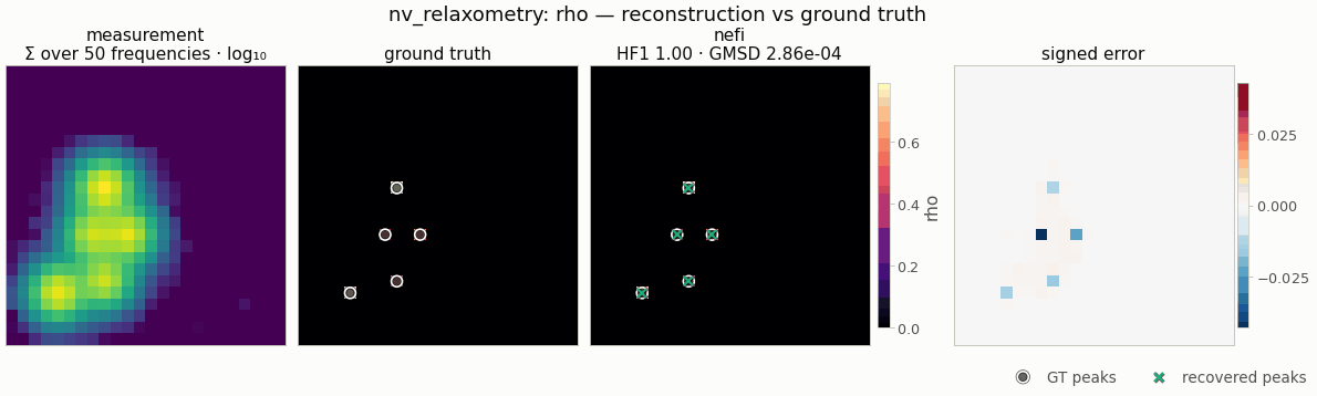
Gallery run (smoke geometry: 24² grid, NV standoff of 3 pixels, 3–5 sources that merge in the measurement; 600 steps, 0.6 s on a CPU): Hungarian F1 1.00.

nefi.instances.nv_relaxometry implements NeTMY (Zhao, Zhong, Hu, de Leon, Allen-Blanchette, Neural Fields for NV-Center Inverse Sensing, arXiv 2605.13988): recovering a sparse spin-source density ρ ≥ 0 and its local Larmor field ω_L from a single noisy magnetic-noise spectrum S_obs(ω, r) read out by a widefield NV-center array at standoff z0. It is label-free and amortization-free: a coordinate neural field is optimized per measurement through a differentiable forward operator.

NVScenes ──► F3 direct simulator (float64) + 1 % noise ──► S_obs (50, 64, 64)
coords ─► annealed Fourier PE (K = 12) ─► MLP 5×320 tanh + skip ─► ρ = softplus(h)·σ(g)
                                                                 ω_L = 1{ρ > 0.3 max ρ}·Bounded(h_ω)
      ─► F2 = (P ∗ ρ)(r) · L(ω; ω_L(r)) ─► D + R_nm + R_ds + ℓ1 + TV ─► AdamW
curriculum 32² (3000 steps) → 64² (7000 steps) ─► energy-anchored scale correction (Eq. 30)

Physics

• Dipolar Green tensor (Eq. 1/8), R = (r − r_src, z0): G_ia(R) = (μ0/4π)(3 R_i R_a − |R|² δ_ia)/|R|⁵, with μ0 = 4π × 10⁻⁷.
• Tensor power kernel (F2, Eq. 2): P(R) = Σ_a |G_az(R)|², which for a z-aligned NV has the closed form (μ0/4π)² (|R|² + 3 z0²)/|R|⁸ (verified in the tests). Its FWHM is ≈ 0.87 z0, so at the paper geometry (20 nm pixels, z0 = 20 nm) the point-spread function is about one pixel wide, and P(1 px)/P(0) = 5/64.
• F2 (tensor/incoherent, linear in ρ): F2 = (P ∗ ρ)(r) · L(ω; ω_L(r)).
• F1 (scalar/coherent, quadratic in ρ): F1 = ((G_zz ∗ ρ)(r))² · L(ω; ω_L(r)).
• F3 (Eq. 11, source-side direct sum): F3 = Σ_s ρ(s) P(r − s) L(ω; ω_L(s)), float64, no FFT.
• Lorentzian (Eq. 13): L(ω; ω_L) = γ²/((ω − ω_L)² + γ²), γ = 0.5 GHz.

Units: units="normalized" (default) divides every channel by the peak of a z-aligned NV, g0 = 2(μ0/4π)/z0³, so max P = max |G_zz| = 1 at every grid resolution (the constant is analytic, not grid-dependent). units="physical" evaluates SI values with domain lengths converted by length_scale (1e-9: domain in nm). Kernels act on per-cell source weights, as in Eq. (11) (no cell-area factor; all fidelities are normalized and the scale correction absorbs it).

Convolutions use FFTConvolution with zero padding and the full 2n − 1 kernel extent, so they are exact linear (non-periodic) convolutions at every curriculum resolution.

Package layout and API

Module	Contents
physics.py	MU0, dipolar_green_tensor(R), DipolarKernels(z0, units, length_scale, nv_axis) (.channels/.power/.nv/.channel, and .power_fn()/.nv_fn()/.channel_fn(a) kernel callables with the FFTConvolution signature (spacing, shape, device, dtype)), power_kernel_fn, gzz_kernel_fn, channel_kernel_fn, lorentzian, frequency_grid
operator.py	NVOperator(domain, freqs, z0, gamma, mode="F2"\|"F1", units, ...) — {rho, omega_L} → (n_freq, H, W), homogeneity 1 (F2) / 2 (F1), at_resolution, output_shape; NVDirectSimulator (F3, fidelity_tag="F3-direct-float64")
losses.py	noise_map(S), normalized_noise_map(S, "max"\|"mean"), DirectDensityLoss (R_ds)
scenes.py	NVScenes (8 paper classes, analytic placement, any shape), PAPER_CLASSES
data.py	NVDataGenerator (noise relative to each sample's dynamic range), downsample_spectrum
__init__.py	NVRelaxometryConfig, NVRelaxometry (registered "nv_relaxometry"), build_problem, make_problem, default_curriculum, METRICS
nefi/metrics/localization.py	gmsd, hungarian_f1, peak_positions, peak_match, sliced_wasserstein ("swd"), wasserstein2_1d

NVRelaxometry methods: domain(), operator(mode), direct_simulator(), scene_generator(), data_generator(), field(seed), losses(measurement), build_problem(measurement, mode, seed), default_curriculum(), build_grid_problem(measurement, mode), baselines() (grid, grid_f1, f1, f2), metrics(), evaluate(result, gt), run(seed, device, scene_class) and compare(seed, scene_class, methods, step_scale) (Tab. 1 on one sample in one call).

Registry entries: instance nv_relaxometry; operators nv_relaxometry (F1/F2) and nv_direct (F3); loss nv_direct_density; scene nv_relaxometry; metrics gmsd, hungarian_f1, sliced_wasserstein/swd.

Paper → code

Paper item	Code	Config field(s)
Eq. (1)/(8) Green tensor	physics.dipolar_green_tensor, DipolarKernels	z0, units, length_scale, nv_axis
Eq. (2) F2, F1	operator.NVOperator(mode=...)	mode
Eq. (9) FFT factorization exact for constant ω_L	tests::test_f2_matches_f3_for_constant_larmor	—
Eq. (11) F3 direct simulator	operator.NVDirectSimulator via NVDataGenerator	data_operator
Eq. (13) Lorentzian, App. A.7	physics.lorentzian	gamma, freq_range, n_freq
App. A.8 χ robustness	tests::test_f2_departs_from_f3_when_larmor_varies_within_kernel	—
Eq. (3) canonical objective / App. E.2 Tikhonov	NVRelaxometry.build_grid_problem	grid_*
Eq. (5) gated softplus	fields.GatedSoftplus	—
Eq. (26) support-masked Larmor head	fields.SupportMasked(Bounded(...), "rho", tau)	tau, larmor_band, larmor_fill
Eq. (27) annealed PE, Tab. 5	fields.NeuralField / FourierFeatures	n_octaves, hidden, depth, skip_at, activation
Tab. 5 optimizer	OptimConfig	optimizer, weight_decay, grad_clip
Tab. 6 two-stage schedule	NVRelaxometry.default_curriculum	steps, lr, lr_decay, lr_min_ratio, coarse_factor, anneal_fraction
Eq. (19) D, log-MSE on max-normalized noise maps	losses.LogMSE(normalize="max", reduce_axes=(0,)) (term log_mse)	w_log_mse, log_eps
App. D.4 R_nm	losses.NormalizedMSE(normalize="mean", reduce_axes=(0,)) (term noise_map)	w_noise_map
App. D.4 R_ds	nv_relaxometry.losses.DirectDensityLoss (term direct_density)	w_direct_density
Tab. 7 ℓ1 (two terms), anisotropic TV	losses.L1 ×2 (sparsity, l1), losses.TV(isotropic=False)	w_sparsity, w_l1, w_tv
App. D.4 stage-2 rebalancing	Stage.loss_weights	stage_loss_weights
Eq. (30), Prop. 1, Eq. (21) scale correction	solve.EnergyScaleCorrection("rho") (uses operator.homogeneity)	scale_correction
App. E.1 scenes (8 classes), noise	scenes.NVScenes, data.NVDataGenerator	scene, counts, separations, margin_z0, amp_range, noise_std
App. E.3 GMSD / Hungarian F1 / SWD / MSE / masked SSIM	metrics.localization, metrics.basic	gmsd_c, match_radius, peak_threshold, swd_projections
Lemma 1 / (P1)	tests::test_power_kernel_fourier_decay_lemma1	—
(P2)+(P3) iter-0 centre bias	tests::test_iter0_center_bias_signature	—

Configuration (NVRelaxometryConfig)

Every number is a config field. The defaults are the paper settings and are spelled out in configs/nv_relaxometry_paper.yaml.

Group	Field	Default	Source
geometry	n, spacing, z0	64, 20 nm, 20 nm	App. E.1
physics	gamma, larmor_band	0.5 GHz, [1.5, 2.5] GHz	App. A.7, E.1
physics	freq_range, n_freq	[1.0, 3.0] GHz, 50	E.1 gives 50 points; range = band ± 2γ (chosen here)
physics	units, length_scale, nv_axis	normalized, 1e-9, (0, 0, 1)	§3.1
data	data_operator, noise_std	F3, 0.01 × dynamic range	§3.1, E.1
data	scene, counts, separations	medium/medium, 1–3 / 4–8 / 9–15, see below	E.1 (as read here)
data	amp_range, margin_z0, min_sep_px, source_width	[0.5, 1], 3 z0, 2 px, 0 (single pixel)	chosen here
inversion	mode	F2	§3.1
field	hidden, depth, skip_at, activation	320, 5 (+ output layer), 3, tanh	Tab. 5
field	n_octaves, tau, larmor_fill	12, 0.3, band centre	Eq. 27, Eq. 26 (fill: see below)
field	out_init_scale, init_seed	0.1, 0	near-uniform init; reproducibility
optimizer	optimizer, weight_decay, grad_clip	adamw, 1e-4, 1.0	Tab. 5
curriculum	steps, lr, lr_decay	(3000, 7000), 1e-3, 0.5	Tab. 6
curriculum	lr_min_ratio, coarse_factor, anneal_fraction, restarts	0.01, 2, 1.0, 1	Tab. 6
curriculum	anneal_reset	true (β → 0 at every stage start)	Tab. 6 (see below)
curriculum	stage_loss_weights	[None, {log_mse: 0, noise_map: 2.0}]	App. D.4
losses	w_log_mse, w_noise_map, w_direct_density	2.0, 0.5, 0.1	Tab. 7
losses	w_sparsity, w_l1, w_tv	1e-2, 1e-3, 1e-3	Tab. 7
losses	w_spectrum	0 (off)	extension (per-frequency fit, identifies ω_L)
losses	log_eps, log_eps_noise_mult	auto, 1.0	Eq. 19 (see below)
post / metrics	scale_correction, match_radius, peak_threshold, swd_projections, gmsd_c	true, 2 px, 5 %, 128, 0.0026	Eq. 30, App. E.3
Tikhonov	grid_steps, grid_lr, grid_weight_decay, grid_l2, grid_tv, grid_init	5000, 5e-3 (Adam), 1e-5, 1e-3, 1e-3, 0.35	App. E.2

Choices where the paper is silent or ambiguous

• Separation classes. Nearest-neighbour distance of every source: close ∈ [2, 3) z0, medium ∈ [3, 5) z0, far ≥ 5 z0 (separations). At 20 nm pixels one z0 is one pixel, so a literal "< 1 z0" class would put two sources in the same pixel. Two 3×3 local maxima need ≥ 2 px, which is also the Hungarian matching radius (≈ ½ w_psf, App. E.3). close scenes are clusters (each new source is placed within the band of an existing one); far scenes are uniform with a minimum distance. The paper's eight classes omit many/medium, but it is accepted.
• Larmor fill outside the predicted support. Eq. (26) writes 0 there. F2 evaluates the Lorentzian at the readout pixel, so a 0 fill multiplies the predicted spectrum around every source (outside the 0.3·max support) by Σ_ω L(ω; 0)/Σ_ω L(ω; 2 GHz) ≈ 1/7. In the runs reported here that lowered Hungarian F1 from 0.93 to 0.65 (32², six samples), so the default fill is the band centre. larmor_fill: 0.0 reproduces the paper literally.
• log-MSE constant. Eq. (19) adds 1e-10 before the log. With additive noise, half of the background pixels of the observed noise map are ≤ 0 and would sit at log10(1e-10) = −10, so the loss would be dominated by noise. log_eps: null (default) uses 1e-10 for noiseless data and otherwise the noise level of the max-normalized noise map (σ·√n_freq / max N_obs ≈ 2.7e-3 at 1 % noise). With 1e-10, HF1 is 0.84 instead of 0.93.
• Depth. Tab. 5 says "6 fully connected layers, hidden 320" and "≈ 4.5 × 10⁵ parameters". Five hidden layers plus the output layer give 444,163 parameters, which matches both statements; six hidden layers would give 5.5 × 10⁵.
• Reductions. L1 and TV are means over pixels (nefi convention), and TV uses unit grid steps (use_spacing=False, Eq. 3). Every data term is scale-invariant, so the absolute ρ scale drifts during optimization and is fixed only by the post-hoc energy correction.
• β reset between stages. Tab. 6 resets β to 0 at the start of stage 2. At β = 0 every Fourier band is gated off, so the MLP output collapses to a smooth function and the stage-1 support is lost. In one traced case all three sources were resolved at the end of stage 1, and the brightest one was never recovered after the reset. anneal_reset: false keeps all bands on after stage 1. On 10 samples (32², 500 + 1000 steps, 5 classes × 2 seeds) it improved every aggregate: HF1 0.898 → 0.951, SWD 0.065 → 0.038, GMSD 0.070 → 0.039, MSE 5.7e-4 → 2.5e-4. It was better or equal on 9 of 10 samples. With the full paper budget the reset recovers (all three paper-scale samples below reach HF1 = 1). The default stays paper-faithful; use anneal_reset: false for short budgets.
• Stage 2. "Replace D by R_nm as the primary fidelity" → {log_mse: 0, noise_map: 2.0}. Keeping D in stage 2 performs the same in 32² runs (HF1 0.94 vs 0.93).
• R_ds is exact only for F1. Under F2 it is a heuristic support proxy, kept at weight 0.1.
• Frequency grid [1, 3] GHz with 50 points. Because every loss acts on frequency-summed maps, ω_L enters the paper objective only through Σ_ω L(ω; ω_L), which varies by ≈ 8 % across the band. ω_L is therefore weakly identifiable (reported as larmor_mae). w_spectrum > 0 adds a per-frequency fit.
• Kernel extent / coarse stage. The coarse stage evaluates F2 on the 32² grid (40 nm cells, kernel re-sampled) against the 2×2 area-averaged spectrum (downsample_spectrum; its noise std is halved accordingly).

Running

Local (CPU, seconds):

python -m pytest -q tests/test_nv_relaxometry.py                 # 20 fast tests, ~5-15 s
python -m pytest -q -m slow tests/test_nv_relaxometry.py         # 32² budget test (≤ 90 s)
python examples/nv_relaxometry.py --config configs/nv_relaxometry_smoke.yaml
# -> runs/nv_relaxometry_smoke/few_close_seed0/{metrics.json,config.yaml,result_netmy.pt,nv_relaxometry.png}

Python API:

from nefi.instances.nv_relaxometry import NVRelaxometry
inst = NVRelaxometry(n=32, hidden=128, depth=4, n_octaves=10, steps=(500, 1000))
out = inst.run(seed=0, scene_class="many/close", device="cpu")
print(out.metrics)                      # gmsd, hungarian_f1, swd, mse, masked_ssim, larmor_mae
tab1 = inst.compare(seed=0, scene_class="medium/medium", methods=("netmy", "f1", "grid", "grid_f1"))

CUDA server (paper settings, ~10k steps per sample; ~3.6 min on a 10-core CPU, much less on GPU):

python examples/nv_relaxometry.py --config configs/nv_relaxometry_paper.yaml --device cuda \
    --scene many/close --seed 0 --out runs/netmy_paper
# the Tab. 1 protocol: loop scenes × seeds; each call runs netmy/f1/grid/grid_f1 on one sample
for s in 0 1 2; do for c in few/close few/medium few/far medium/close medium/medium medium/far \
    many/close many/far; do python examples/nv_relaxometry.py \
    --config configs/nv_relaxometry_paper.yaml --device cuda --seed $s --scene $c; done; done

YAML layout: an instance: block (type: nv_relaxometry plus any NVRelaxometryConfig field, buildable with nefi.build("instance", cfg["instance"])) and a run: block (seed, device, methods, out). --set key=value overrides any field, and --steps-scale scales every curriculum.

Expected outputs

Validation (fast tests; numbers from this implementation):

Check	Result
F2 (FFT) vs F3 (direct), constant ω_L, 64²	rel. error 2.5e-16 (float64 F2), 2.3e-7 (float32 F2)
F2 vs F3, per-source ω_L as in the benchmark data	5.6e-2 (the inverse-crime gap the benchmark relies on)
F2 vs F3, χ = 0.1 / 0.3 / 1.0 / 1.08 (in-band sinusoidal ω_L, 64²)	1.2e-3 / 4.2e-3 / 2.3e-2 / 2.6e-2 (paper, App. A.8: 2.6e-2 at χ ≈ 0.3, 1.6e-1 at χ ≈ 1.08, with its own χ definition)
Homogeneity F2 / F1	max rel. deviation 4e-15 / 9e-13
Lemma 1	radial |P̂(k)| strictly decreasing; P̂(k)·e^{k z0}/(1 + k z0)³ ≤ P̂(0); tail log-slope ≈ −0.77/z0
Iter-0 gradient, uniform ρ, F2	centre/outer-ring 112× (32²), argmax at the grid centre (paper: 18.29×); under F1 0.33× (no centre bias)
Scale correction ρ⋆/3	recovers ρ⋆ exactly (α = 3 under F2 and, by the √ rule, under F1)

Smoke / gallery run (configs/nv_relaxometry_smoke.yaml): a deliberately ill-posed geometry. The NV standoff is 3 pixels (z0 = 60 nm on a 24² grid of 20 nm pixels; paper: 1 pixel), so the point-spread function is ≈ 2.6 px wide, and the scene class few/close is redefined for this geometry (separations: close = [1.0, 1.5) z0 = 3–4.5 px, counts: few = 3–5): the 3–5 sources merge into one blob in the measured noise map (drawn log-scaled, NVRelaxometry.viz_hints) and the inversion has to separate them. Because the observed map is blurred over 3 px, the direct-density proxy R_ds — which pulls ρ² toward that map — is switched off (w_direct_density: 0). At 40 + 60 steps (~1 s) Hungarian F1 over seeds 0–9 is 0.91, 0.86, 0.91, 0.8, 0.8, 0.75, 1.0, 0.83, 0.89, 0.89 (mean 0.86); at the gallery's 600 steps (--budget 0.1, ≈ 1–2 s) it is 1.0 on nine seeds and 0.91 on one (seed 0: every merged source recovered as a single pixel, GMSD 3e-4). The Tikhonov grid baseline (200 steps) finds none of the merged sources on seed 0 (Hungarian F1 0). At a 1-pixel standoff with few/far scenes the noise map already shows every source as a separate dot, which is why the smoke preset uses the harder geometry.

Paper settings (configs/nv_relaxometry_paper.yaml: 64², 3000 + 7000 steps, 4.4e5-parameter MLP, β reset, F3 data with 1 % noise), NeTMY under F2, seed 0:

Scene	HF1 ↑	SWD ↓	GMSD ↓	masked SSIM ↑
few/far	1.00	0.055	1e-4	1.000
medium/medium	1.00	0.006	5e-4	1.000
many/close	1.00	0.006	9e-4	1.000

On a 10-core CPU a paper-scale run takes ≈ 3.6 min (9 ms/step at 32², 27 ms/step at 64²). Density MSE after scale correction is < 1e-4 in all three. The full 7000-step stage 2 recovers from the β reset; the reset penalty above is a reduced-budget effect.

Reduced-budget cross-fidelity comparison (32², hidden 128, depth 4, K = 10, 500 + 1000 steps; F3 data; seed 0 on few/far, medium/medium, many/close):

Method	HF1 ↑	SWD ↓	GMSD ↓	MSE ↓
NeTMY (F2)	0.90	0.083	0.071	5e-4
NeTMY (F1)	0.40	0.159	0.236	5e-3
Tikhonov (F2)	0.92	0.129	0.090	1.8e-3
Tikhonov (F1)	0.14	0.194	0.191	1.1e-2

As in Tab. 1, every method improves when moving from F1 to F2, and NeTMY is best on SWD, GMSD and MSE. At this geometry the PSF is about one pixel wide, which makes sparse scenes comparatively easy, so free-density Tikhonov remains competitive on Hungarian F1.

Known failure modes and limitations

From NeTMY App. E.10, all reproducible with this instance:

• Cross-shaped artifacts on dense scenes (many sources within w_psf; the (P4) anisotropic explanation). Mitigations: nefi.losses.Laplacian or isotropic TV (slightly worse MSE).
• High-frequency leakage on small clusters at full β = K (only ℓ1 plus the gate suppress it). Mitigations: raise w_sparsity, lower n_octaves, or use anneal_fraction < 1.
• Centred-minimum trapping from an unlucky initialization (≈ 5 % of samples in the paper). Use restarts > 1 (best final data loss wins) or several seeds (nefi.ensemble).

Limitations of this implementation:

• ω_L is only weakly constrained by the paper's frequency-summed losses (see above).
• The ρ scale is unidentifiable during optimization. The energy correction is exact in the noiseless limit, but with noise it inherits E_ε/E⋆ and any shape error (App. B.3).
• F3 builds dense n_pix × n_src blocks: sparse scenes cost milliseconds, a fully dense 64² ρ about 4 s on CPU (float64).
• units: physical puts the power kernel peak at ≈ 6e32 (SI, z0 = 20 nm). A dense O(1) density sums to ≈ 1e38 over a 50 × 64² spectrum, close to float32 overflow (3.4e38), and F1 grows as ρ². Use the normalized default, or run the solver in float64 (Solver(dtype=torch.float64)) or rescale ρ, when working in physical units.
• Tiny budgets (≤ 100 steps) need a larger learning rate than the paper (the smoke config uses 0.02).