photoacoustic3d — 3-D photoacoustic tomography from a planar sensor array

At a glance
Problem	3-D photoacoustic tomography from a planar sensor array on the top face (limited view)
Unknown	initial pressure p0 ≥ 0 (softplus head), 48 × 48 × 32 voxels over 12 × 12 × 8 mm
Physics	3-D wave equation with zero initial velocity: leapfrog, sponge layer, Gaussian sensor bandwidth
Measurement	pressure traces of 16 × 16 point sensors + 2 % noise; data on a 2× grid in float64
Difficulty classes	vessels, spheres
Baselines	time_reversal, grid
Metrics	PSNR · slice SSIM · MSE
Run	nefi run photoacoustic3d --smoke · full: nefi run configs/photoacoustic3d_full.yaml --device cuda

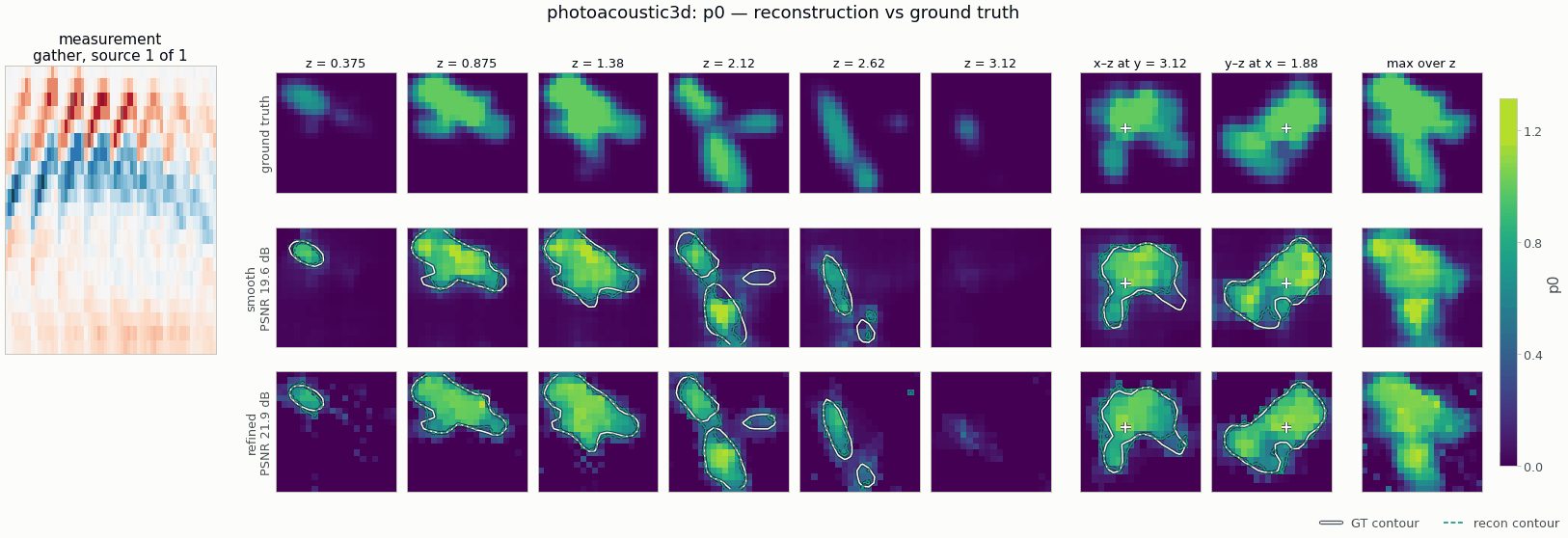
Gallery run (20 × 20 × 14, 8 × 8 sensors; 400 steps, 8.4 s on a CPU): PSNR 19.6 dB; edge refinement accepted, IoU 0.73 → 0.80. Rotate it in the 3-D showcase.

Recover the initial pressure p0(x, y, z) ≥ 0 (the optical energy absorbed from a short laser pulse) of a tissue slab from the pressure traces of a planar n_sx × n_sy array of point sensors on its top face:

∂²p/∂t² = c² Δp,    p(x, 0) = p0(x),    ∂p/∂t(x, 0) = 0        (homogeneous, known c = 1.5 mm/µs)
y_s(t_j) = [h ∗ p](x_s, t_j) + n       (h: sensor bandwidth, Gaussian low-pass at sensor_fc)

A planar array sees the object from one side only (limited view): structures whose boundaries are parallel to the viewing direction produce no signal on the array, and the classical time-reversal image is blurred and streaked. The map p0 ↦ y is linear (homogeneity = 1).

PAT3DScenes (vessels | spheres) ─► leapfrog on a 2× grid (float64) + sensor low-pass ─► traces (n_sensors, n_t) + 2 % noise
coords ─► annealed Fourier PE (3-D) ─► MLP ─► Softplus ─► p0 ─► WaveInitialConditionOperator (3-D, sponge) ─► SensorBandwidth
       ─► MSE + λ·TV₃D ─► two-stage multiscale (½ res: 16× cheaper wave solves) ─► PSNR / slice-SSIM / MSE

from nefi.instances.photoacoustic3d import Photoacoustic3D

inst = Photoacoustic3D(preset="smoke")       # 5 × 5 × 3.5 mm at 0.25 mm voxels, 8×8 sensors
out = inst.run(seed=0, device="cpu")
tr = inst.time_reversal(out.measurement)    # k-Wave-style time reversal (closed form)

CLI: nefi run photoacoustic3d --smoke, nefi run configs/photoacoustic3d_full.yaml --device cuda. Example: python examples/photoacoustic3d.py [--set scene=spheres] writes photoacoustic3d.png (depth slices, max-intensity projections over depth and in x-z of GT / NF / time reversal, and the measured vs predicted trace gathers) under runs/photoacoustic3d_smoke/.

Forward model

• Photoacoustic3D.wave_operator() — nefi.physics.wave.WaveInitialConditionOperator in 3-D: leapfrog in time with p⁻¹ = p¹ (zero initial velocity), centered 2nd- (default) or 4th-order Laplacian as one conv3d per step, a sponge absorbing layer of absorb_width mm around the slab (the 3-D solver has no PML), CFL-limited substeps between the trace samples dt_obs, sensors sampled by trilinear interpolation at fixed physical positions and times — so the output (n_sensors, n_t) is resolution independent and every curriculum stage fits the same traces. Gradients: autodiff through the unrolled scheme (the discrete adjoint; grad_mode="checkpoint" for larger grids).
• SensorBandwidth(inner, dt_obs, f_cutoff) — the transducers' finite bandwidth, a zero-phase Gaussian low-pass exp(−½ (f/f_c)²) along time (zero-padded FFT). It is part of the physics of both the data generator and the inversion and band-limits the traces to what the grid propagates accurately: with 0.25 mm voxels the native-vs-2× model mismatch is 4.5 % of the peak trace for ideal sensors and 2.0–2.4 % at f_c = 1 MHz (1.4–1.7 % at 0.75 MHz; 1.0 % with the 4th-order stencil).

Scenes and data

PAT3DScenes (physical mm, smooth tanh edges of edge_width, cell-averaged): vessels (2–4 random vessel trees — persistent random walks running mostly parallel to the skin with one branch each — of radius 0.3–0.6 mm; the canonical PAT angiography target and a hard limited-view case) and spheres (3–6 absorbing balls of radius 0.6–1.5 mm). Inverse-crime guard: the traces are simulated on a 2× finer grid in float64 (gen_order stencil; gen_order=4 adds a different stencil at ≈ 5× the data-generation cost) with the same sensor response, plus 2 % relative noise (fidelity_tag = "wave-ic-o2-2x-float64-lp1.0" vs "wave-leapfrog-ic-o2-sponge-lp1").

Configuration (Photoacoustic3DConfig) and presets

field	default	smoke	meaning
extent, grid	(12, 12, 8) mm, (48, 48, 32)	(5, 5, 3.5), (20, 20, 14)	slab and grid (0.25 mm voxels in both)
sound_speed	1.5 mm/µs		homogeneous, known
sensor_grid, sensor_span, sensor_depth, sensor_fc	(16, 16), 0.9, 0.0, 1.0 MHz	(8, 8)	planar array on the top face
t_max, dt_obs	12 µs, 0.25 µs	5 µs	records
order, absorbing, absorb_width, absorb_R, courant, grad_mode	2, sponge, 1.0 mm, 1e-3, 0.9, autograd		solver
noise_std, supersample, gen_order	0.02, 2, 2		data
scene, vessel_radius, sphere_radius, edge_width, depth_range	vessels, …		scenes
init_value, tv, tv_eps, l1	0.02, 1e-4, 1e-3, 0		prior
hidden, depth, skip_at, n_octaves, activation	128, 4, 2, 5, tanh	64, 3, 2, 4	neural field
steps, lr, lr_decay, anneal_fraction, min_coarse	(300, 500), 1e-2, 0.5, 0.3, 8	(150, 50), 2e-2	curriculum
grid_lr, tr_mode	5e-2, dirichlet		baselines

The smoke preset is a cropped field of view at the same voxel size as the full configuration, so the wave physics per voxel (points per wavelength, CFL, sponge thickness) is identical; most of its steps run on the coarse stage (16× cheaper: 8× fewer cells, 2× fewer time steps). Presets: smoke, spheres, default. Configs: configs/photoacoustic3d_smoke.yaml, configs/photoacoustic3d_full.yaml (48×48×32, 16×16 sensors, 750 + 1250 steps).

Baselines (Photoacoustic3D.baselines())

grid (free voxels, same objective) and time_reversal (closed form through the DirectSolver: nefi.physics.wave.time_reversal, the k-Wave-style Dirichlet re-emission of the time-reversed traces at the sensor cells, Treeby & Cox 2010; tr_mode="adjoint" gives the exact discrete adjoint / back-projection instead), clipped to p0 ≥ 0.

Validation (tests/test_photoacoustic3d.py, ≈ 6 s)

check	result
forward cost (one CPU thread; 3-D wave, 2nd order)	smoke 20×20×14 (60 leapfrog steps): 41 ms forward, 127 ms forward + backward; 24×24×16 (72 steps): 76 / 212 ms; 48×48×32 (144 steps): 0.68 / 2.3 s
linearity A(2a − 0.5b), exact adjoint ⟨Aa, y⟩ = ⟨a, Aᵀy⟩ (float64)	≤ 1e-10, ≤ 1e-9 relative
sensor low-pass: zero phase in the passband, 4 MHz tone at f_c = 1 MHz	≤ 0.05 / ≤ 1e-3
scenes: avg_pool(2× render) = native	≤ 1e-5
native model error vs 2× data (noise-free, relative to the peak trace)	≈ 2 % (asserted < 3.5 %)
time reversal	correlates with the ground truth (ρ > 0.3); DirectSolver result = closed form

The 3-D forward stays far below the 1 s-per-call budget on CPU at 24×24×16 (76 ms), so the full 3-D version (rather than a thin-slab / 2-D-sensor fallback) is shipped.

Inversion (seed 0, smoke preset, 2 % noise; PSNR dB / SSIM):

scene	time reversal	neural field (200 steps, ≈ 4 s on 4 threads)
vessels	10.9 / 0.317	17.9 / 0.581
spheres	9.1 / 0.307	15.5 / 0.524

The neural field with TV recovers the vessel topology and the depth of the structures that time reversal smears into a blob (limited view + band-limited sensors); the reconstruction is still blurred at depth (limited view) and under-converged at the smoke budget (data loss ≈ 8× the noise floor).

Notes and limitations

• Homogeneous, known sound speed; no acoustic attenuation, no heterogeneous c (the solver supports a c map — joint p0/c recovery is a natural extension).
• Point sensors with a Gaussian low-pass (no directivity, no finite element size, no band-pass zero at DC).
• The 3-D sponge layer (1 mm ≈ 0.7 dominant wavelengths at 1 MHz) reflects a little; the data generator uses the same physical layer, so this is shared physics, not an inverse crime.
• Memory: grad_mode="autograd" stores every leapfrog state (≈ n_steps × padded cells); use grad_mode: checkpoint for 96³-class grids.