deconvolution3d — fluorescence-microscopy z-stack deconvolution

At a glance
Problem	Widefield fluorescence z-stack deconvolution with an axially elongated PSF
Unknown	fluorophore density x ≥ 0 (softplus head), 64 × 64 × 32 anisotropic voxels
Physics	3-D FFT convolution with a Gaussian PSF, σz = 3 σxy, in physical µm
Measurement	blurred z-stack + Gaussian noise or Poisson photon counts; data on a 2× grid in float64
Difficulty classes	filaments, puncta, cells
Baselines	richardson_lucy, wiener3d, grid, deep_decoder
Metrics	PSNR · slice SSIM · MSE
Run	nefi run deconvolution3d --smoke · full: nefi run configs/deconvolution3d_full.yaml

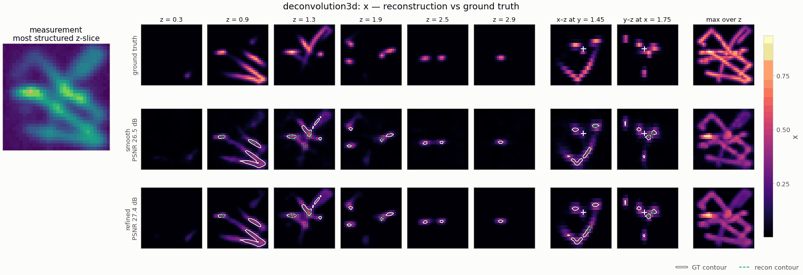
Gallery run (32 × 32 × 16; 800 steps, 12.5 s on a CPU): PSNR 26.5 dB; edge refinement accepted, IoU 0.65 → 0.71.

Recover the non-negative fluorophore density x(x, y, z) from a widefield z-stack blurred by the microscope's 3-D point-spread function:

y = h ∗ x + n              (Gaussian noise, relative std noise_std)
y ~ Poisson(peak · (h ∗ x) + background)      (photon counts, noise = "poisson")

The PSF is the Gaussian approximation of the widefield PSF (Zhang, Zerubia & Olivo-Marin, Appl. Opt. 46, 2007) with the classic axial elongation σ_z = psf_axial_ratio · σ_xy (default 3) in physical µm. Camera pixels (pixel_size, default 0.1 µm) and z-steps (z_step, default 0.2 µm) are independent, so the voxels are anisotropic like a real stack.

Deconvolution3DScenes (filaments | puncta | cells) ─► PSF blur on a 2× grid (float64), area-averaged ─► stack + noise
coords ─► annealed Fourier PE (3-D) ─► MLP ─► Softplus ─► x ─► FFTConvolution(Gaussian PSF(spacing)) [× peak + bg]
       ─► MSE | Poisson NLL + λ·TV₃D + μ·ℓ1 ─► two-stage multiscale ─► PSNR / slice-SSIM / MSE

from nefi.instances.deconvolution3d import Deconvolution3D

inst = Deconvolution3D(preset="smoke")         # 32×32×16 stack (3.2 µm cube), 150 + 250 steps
out = inst.run(seed=0, device="cpu")
rl = inst.richardson_lucy(out.measurement)     # the classical ML-EM reference
wiener, snr = inst.wiener_reconstruction(out.measurement)

CLI: nefi run deconvolution3d --smoke, nefi run configs/deconvolution3d_full.yaml, nefi bench deconvolution3d --smoke --methods neural,richardson_lucy,wiener3d,grid. Example: python examples/deconvolution3d.py [--set scene=puncta --set l1=1e-3 | --set noise=poisson] writes deconvolution3d.png (z-slices, the max-intensity projection and an x-z MIP of GT / blurred / RL / NF) under runs/deconvolution3d_smoke/.

Forward model

Deconvolution3D.blur() is the N-D nefi.operators.FFTConvolution with the kernel function gaussian_kernel_fn((σ_xy, σ_xy, σ_z)) — sampled at the grid spacing of every curriculum stage and of the data-generation grid, unit sum, zero-padded linear convolution (psf_extent="full": exact linear support 2n − 1; "same": kernel truncated to the stack, 3–4× cheaper, fine for compact PSFs). For Poisson data the operator is Nuisance(blur, init_gain=peak_counts, init_offset=background_counts) with frozen gain/offset, i.e. expected counts. The full-extent Gaussian kernel is symmetric, so the zero-padded blur is self-adjoint (tested).

Scenes (Deconvolution3DScenes, physical µm, cell-averaged)

• filaments — 3–6 persistent random walks (mostly in-plane, like cytoskeletal fibres) with a Gaussian cross-section of filament_sigma = 0.06–0.09 µm;
• puncta — 12–30 sub-voxel point sources of width puncta_sigma = 0.04–0.07 µm rendered as exact erf cell averages (no aliasing at any resolution) — the regime where ℓ1 helps (preset puncta: l1 = 1e-3);
• cells — 1–2 ellipsoidal cells with a bright membrane shell (membrane_width 0.06 µm), dim cytoplasm, a nucleus and a few vesicles.

Inverse-crime guard: the stack is blurred on a 2× finer grid in float64 (the PSF re-sampled at the fine spacing) and area-averaged onto the camera voxels (fidelity_tag = "blur3d-2x-float64" vs "blur3d-1x-float32"); the rendering sub-grid is shared, so the native ground truth is the exact area average of the fine one.

Classical references (nefi.instances.deconvolution3d.classical)

• wiener3d(image, psf, snr, pad, clip, boundary="normalize") — the N-D Wiener filter of the 2-D instance (boundary normalization by the blurred indicator, replicate padding of a quarter of each axis); wiener3d_discrepancy picks the SNR by Morozov's discrepancy principle;
• richardson_lucy(counts, blur, n_iter, gain, background) — ML-EM for Poisson data (Richardson 1972; Lucy 1974) with the exact adjoint of the zero-padded blur (autograd), a known background, rl_iters iterations (early stopping is the regularizer). It preserves positivity and the predicted flux Σ A x = Σ y.

Configuration (Deconvolution3DConfig) and presets

field	default	smoke	meaning
n, n_z, pixel_size, z_step	64, 32, 0.1, 0.2	32, 16	stack size, voxel (µm)
scene, render_factor, filament_sigma, puncta_sigma, membrane_width	filaments, 2, …		scenes
psf_sigma_xy, psf_axial_ratio, psf_extent	0.12, 3.0, full		PSF (µm)
noise, noise_std, peak_counts, background_counts, supersample	gaussian, 0.01, 200, 2, 2		data
head, init_value, data_loss	softplus, 0.05, auto		auto = MSE / Poisson NLL
tv, tv_eps, l1	1e-4, 1e-3, 0		regularizers
hidden, depth, skip_at, n_octaves, activation	128, 4, 2, 6, tanh	64, 3, 2, 5	neural field
steps, lr, lr_decay, anneal_fraction, min_coarse	(600, 1200), 1e-2, 0.5, 0.3, 8	(150, 250), 2e-2	curriculum
grid_lr, dd_*, wiener_snr, wiener_tau, rl_iters	5e-2, …, 0, 1, 30		baselines

Presets: smoke, poisson (100 photons at unit intensity, background 2), puncta (scene + ℓ1), default. Configs: configs/deconvolution3d_smoke.yaml, configs/deconvolution3d_full.yaml (64×64×32, psf_extent: same, 1500 + 3000 steps).

Baselines (Deconvolution3D.baselines())

grid (free voxels, same objective), wiener3d and richardson_lucy (closed form through the DirectSolver), deep_decoder (3-D).

Validation (tests/test_deconvolution3d.py, ≈ 20 s)

check	result
sampled PSF second moments vs σ_xy, σ_z	within 5 % (unit sum to 1e-10)
point source: axial vs lateral spread	σ_z / σ_xy = 3
linearity; self-adjointness of the full-extent blur	≤ 1e-10 relative
scenes: avg_pool(2× render) = native (all classes)	≤ 1e-5
model error of the native operator vs the 2× data (noise-free)	≤ 5e-4 of the max (filaments), ≤ 1.3e-3 (puncta) — far below the noise
Wiener on a periodic blur of a band-limited field (SNR 1e8)	relative error ≤ 1e-3
RL: positivity, predicted-flux conservation	≥ 0, Σ A x / Σ y − 1 ≤ 1 %

Operator cost (one thread): 32×32×16 blur 5.9 ms forward / 17 ms forward + backward (full), 1.4 / 4.6 ms (same); 64×64×32: 48 / 138 ms (full), 16 / 46 ms (same).

Inversion (seed 0, 1 % Gaussian noise, 32×32×16; PSNR dB / SSIM):

scene	blurred	Wiener (discrepancy)	Richardson–Lucy (30 it)	neural field, smoke (400 steps)	neural field, 900 steps
filaments	22.0 / 0.658	24.4 / 0.696	25.7 / 0.810	25.2 / 0.789	26.8 / 0.868
cells	21.3	24.2 / 0.716	24.4 / 0.781	23.6 / 0.761	25.4 / 0.827
puncta	29.8	31.8 / 0.859	32.3 / 0.906	31.4 / 0.900	—

At the smoke budget the neural field is on par with Richardson–Lucy (the smoke run stops at ≈ 3× the noise floor of the data loss); with 900 steps it beats RL by 1–1.1 dB / +0.05 SSIM on filaments and cells. RL remains a strong reference for sparse puncta.

Notes and limitations

• Gaussian PSF only (no Gibson–Lanni / Born–Wolf model, no depth-dependent aberrations, no missing-cone structure); swap blur() for a tabulated PSF (tensor kernel) to use a measured one.
• The anisotropic TV uses physical spacing (µm), so the axial and lateral gradients are weighted consistently; there is no separate axial weight.
• With noise="poisson" and data_loss="mse" the MSE weight is 1/peak² (image units).