deconvolution — 2-D image deblurring

At a glance
Problem	2-D image deblurring with a known Gaussian, linear-motion or out-of-focus PSF
Unknown	image x ≥ 0 (softplus head), 64²
Physics	zero-padded FFT convolution; the PSF is a function of the grid spacing, so every stage sees the same physical blur
Measurement	blurred image + Gaussian noise or Poisson photon counts; data from the PSF on a 2× grid in float64
Difficulty classes	phantom, smooth, sparse_dots
Baselines	grid (+ TV), admm, deep_decoder, gaussian_splat, wiener
Metrics	PSNR · SSIM · MSE
Run	nefi run deconvolution --smoke · full: nefi run configs/deconvolution_full.yaml

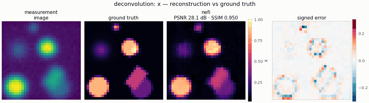
Gallery run (32², 450 steps, 0.4 s on a CPU): PSNR 28.1 dB, SSIM 0.95.

Recover a non-negative image x on [0, extent]² from a blurred, noisy observation

Gaussian noise:  y = k ∗ x + n,             n ~ N(0, (noise_std · max(k ∗ x))²)
Poisson noise:   y ~ Poisson(peak · (k ∗ x) + background)       (photon counts)

with a Gaussian (psf_sigma), linear-motion (motion_length, motion_angle) or out-of-focus disk (disk_radius) point-spread function given in physical units.

from nefi.instances.deconvolution import Deconvolution
inst = Deconvolution(n=64, scene="phantom", psf="motion", noise="poisson")
out = inst.run(seed=0)                  # generate -> invert -> evaluate (RunOutput)
out.metrics                             # {"psnr", "ssim", "mse"}

CLI: nefi run deconvolution --smoke, nefi run configs/deconvolution_full.yaml, nefi bench configs/deconvolution_full.yaml --n 8 --seeds 0,1,2. Example: python examples/deconvolution.py [--config ...] [--set psf=disk].

Physics and discretization

• Operator — FFTConvolution(psf_fn, domain, periodic=False): zero-padded linear convolution ("same" output), FFT kernel cache per resolution. The PSF is a kernel function of the grid spacing (nefi.instances.deconvolution.psf): the Gaussian is sampled analytically, the motion segment is splatted bilinearly with 8 samples per cell, the disk is anti-aliased with 8×8 sub-samples; all are normalized to unit sum. Every curriculum stage therefore sees the same physical PSF. Poisson mode wraps the blur in a fixed Nuisance gain/offset (peak_counts, background_counts) so the prediction is in expected counts.
• Data generation (inverse-crime guard) — BlurDataGenerator: the same PSF evaluated on a supersample = 2× finer grid in float64, the blurred image area-averaged onto the detector grid, then Gaussian or Poisson noise from the scene's numpy generator (fidelity_tag = "blur-2x-float64"; the inversion operator is tagged "blur-1x-float32").
• Scenes (DeconvolutionScenes, values in [0, 1], analytic and rendered as cell averages so every grid sees the same scene): phantom (piecewise-constant disks and rotated rectangles with random contrast, soft blobs, a few sparse dots), smooth (broad blobs + low-frequency texture), sparse_dots (6-15 near-point sources of width dot_cells native cells).

Prior, objective and curriculum

Neural field (hidden × depth tanh MLP, skip at skip_at, annealed Fourier features with n_octaves) with a Softplus (default) or Bounded(0, 1) head. Losses: data = MSE (Gaussian) or Poisson NLL weighted by 1/peak_counts (so regularizer weights are in image units), tv = isotropic TV (NeFTY Eq. 22, physical-spacing differences, tv_eps), l1 (off by default; use it for sparse_dots). Two-stage multiscale curriculum n/2 → n with the NeTMY schedule (cosine LR per stage, β reset per stage, second stage at lr · lr_decay).

Configuration (DeconvolutionConfig)

field	default	meaning
n, extent	64, 1.0	grid size, physical side length
scene	phantom	phantom | smooth | sparse_dots
psf	gaussian	gaussian | motion | disk
psf_sigma	0.02	Gaussian std (1.28 px at n = 64)
motion_length, motion_angle	0.1, 30.0	motion blur length, angle in degrees from axis 0
disk_radius	0.04	defocus radius
noise	gaussian	gaussian | poisson
noise_std	0.01	relative Gaussian noise std
peak_counts, background_counts	200, 1	Poisson exposure and dark counts
supersample	2	data-generation grid factor
dot_cells	0.7	width of sparse_dots sources in native cells
head, init_value	softplus, 0.05	softplus | bounded (Bounded(0, 1))
data_loss	auto	auto (MSE / Poisson NLL by noise model) | mse | poisson_nll
tv, tv_eps, l1	1e-4, 1e-3, 0	regularizer weights
hidden, depth, skip_at, n_octaves, activation	128, 4, 2, 7, tanh	neural field
steps, lr, lr_decay, anneal_fraction	(400, 800), 2e-2, 0.5, 1.0	curriculum
grid_lr, grid_l2	5e-2, 0	grid baseline LR and optional extra ℓ2 (Tikhonov) weight
dd_lr, dd_width, dd_stages	5e-3, 64, 5	Deep Decoder baseline
splat_lr, splat_primitives, splat_max_primitives	3e-2, 64, 128	Gaussian-splat baseline
admm_mu, admm_l1, admm_lr, admm_inner, admm_outer, admm_tol, admm_adaptive	0.1, 1e-3, 2e-2, 20, 60, 1e-3, true	ADMM baseline
wiener_snr, wiener_tau	0 (auto), 1.0	fixed Wiener SNR, or discrepancy factor for the automatic choice

Configs: configs/deconvolution_smoke.yaml (32², ~5 s CPU), configs/deconvolution_full.yaml (64², 1200 + 2400 steps, full-size baselines; GPU recommended).

Baselines (Deconvolution.baselines())

grid (free pixels with the same losses), deep_decoder, gaussian_splat (designed for sparse_dots), admm (grid + ℓ1/box ADMM, box from the head range) and wiener: the classical Wiener filter X = H* Y / (|H|² + 1/snr) with the zero-padding boundary handled by dividing by the blurred domain indicator k ∗ 1_Ω and replicate padding, and the SNR chosen by Morozov's discrepancy principle (wiener_discrepancy; within ~1-2 dB of the best fixed SNR in the checks). See docs/baselines.md for what each baseline means and when the comparison is fair.

Validation

tests/test_deconvolution.py (≈ 8 s): unit-sum, centered, physically scaled PSFs (a 2× finer grid doubles the Gaussian width in pixels; motion at 90° is the transpose of 0°); scene values in [0, 1] and exact fine→native area consistency; Poisson data are non-negative integers with the expected mean; the Wiener filter inverts a circular blur exactly and deblurs instance data by

2 dB; inverse-crime tags differ; the smoke inversion beats the blurred input by > 2 dB; the Poisson-NLL path runs; every baseline builds and solves.

Measured on a CPU (seed 0, phantom, Gaussian PSF, 1 % noise):

setting	blurred	Wiener	neural field	grid + TV	Deep Decoder	Gaussian splat	ADMM (ℓ1)
32², smoke (450 steps)	21.03 / 0.805	24.96 / 0.833	28.05 / 0.950 (4.5 s)	29.07 / 0.971 (0.7 s)	24.12 / 0.876	23.45 / 0.898	25.16 / 0.810
64², 300 + 600 steps	24.26 / —	27.65 / 0.781	33.60 / 0.981 (22 s)	35.13 / 0.987 (1.5 s)	29.66 / 0.956	27.26 / 0.922	26.96 / 0.628

(PSNR dB / SSIM.) On this well-conditioned linear problem the TV-regularized free grid — the MAP estimate of the same objective — is a very strong baseline and the neural field is competitive with it, far ahead of Wiener, the Deep Decoder and the sparse priors (which lack TV and fit piecewise-constant shapes poorly). On sparse_dots with an ℓ1 objective the ranking changes (docs/baselines.md). These are single-seed numbers; use nefi bench for CIs.

Notes and limitations

• The PSF is known; blind deconvolution would add the kernel as a nuisance parameter.
• Poisson NLL on area-averaged counts at the coarse stage is a slightly mis-specified likelihood (averaged counts are not Poisson); the minimizer is unaffected.
• The Wiener filter is a single global SNR (flat noise-to-signal ratio); boundary handling assumes the image is locally smooth at the border.